8.8 SPECTRAL ANALYSIS
![]()
INTRODUCTION |
When a beam of light falls on your eyes or you hear a tone, a signal accrues that can be regarded as a function of time y(t). With a single spectral color or a pure tone, it consists of a sinusoidal oscillation with the amplitude A and frequency f, expressed mathematically [more... It does not start counting the time at the beginning of the sine wave, one needs to take into account a phase shift]:
|
SPECTRUM OF A SOUND, OVERTONES |
The sinusoidal frequency components that are present are important for the typical tone color of a voice or a musical instrument. A strictly periodic sound consists of the fundamental and the overtones, whose frequencies are integer multiples of the frequency of the fundamental. If you plot the amplitude of the frequency components in a graph, you get the spectrum of the sound. You can determine the spectrum with a device called a spectral analyzer. TigerJython can determine the spectrum using a famous algorithm called the Fast Fourier Transform (FFT). In order to perform the FFT, you give the function fft(samples, n) a list samples that contains the temporally equidistant sample values and the number n of samples that should be used for the FFT from the beginning of the list. These n/2 return values at the distance r "populate" the frequency range from 0 to n/2*r = fs/2, or in a nutshell: The FFT provides the spectrum from 0 to fs/2 at a sampling frequency of fs. A CD with a typical sampling frequency where fs = 44100 Hz corresponds to a spectrum up to 22050 Hz, which covers the entire audible range of humans.
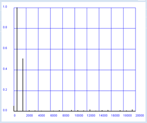
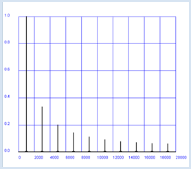
from soundsystem import * from gpanel import * def showSpectrum(text): makeGPanel(-2000, 22000, -0.2, 1.2) drawGrid(0, 20000, 0, 1.0, 10, 5, "blue") title(text) lineWidth(2) r = fs / n # Resolution f = 0 for i in range(n // 2): line(f, 0, f, a[i]) f += r fs = 40000 # Sampling frequency n = 10000 # Number of samples samples = getWavMono("wav/doublesine.wav") openMonoPlayer(samples, fs) play() a = fft(samples, n) showSpectrum("Audio Spectrum") |
MEMO |
As you imagine (and hear) you find the frequencies 500 Hz and 1.5 kHz with an amplitude ratio of 1 : 1/2. There are some additional disturbance components. The frequency 0 corresponds to a constant signal component (offset). You now have a feudal spectrum analyzer in front of you, with which you can examine the fundamentals and overtones of musical instruments, human sounds, or animal sounds with. You will already find the sound of a flue ("wav/flute.wav") and an oboe ("wav/oboe.wav") in the distribution, whose sound characteristics are very different. |
|
SPECTRA FOR SELF-DEFINED FUNCTIONS |
According to the theorem of Fourier, every periodic function with the frequency f can be represented as superpositions of sine functions with the frequencies f, 2*f, 3*f, etc. (Fourier series).
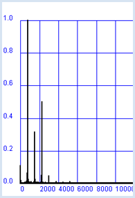
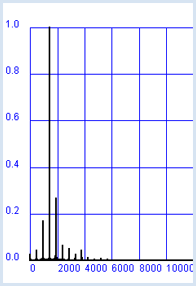
from soundsystem import * from gpanel import * def showSpectrum(text): makeGPanel(-2000, 22000, -0.2, 1.2) drawGrid(0, 20000, 0, 1.0, 10, 5, "blue") title(text) lineWidth(2) r = fs / n # Resolution f = 0 for i in range(n // 2): line(f, 0, f, a[i]) f += r n = 10000 fs = 40000 # Sampling frequency f = 1000 # Signal frequency samples = [0] * 120000 # sampled data for 3 s t = 0 dt = 1 / fs # sampling period for i in range(120000): samples[i] = square(1000, f, t) t += dt openMonoPlayer(samples, 40000) play() a = fft(samples, n) showSpectrum("Spectrum Square Wave") |
MEMO |
The experiment shows that the spectrum of a rectangular function consists of the odd multiples of the fundamental frequency and where the amplitudes of the spectral components behave as 1, 1/3, 1/5, 1/7, etc. However, you will never be able to find out experimentally that the spectral parts theoretically stretch until ad infinitum. |
SONOGRAM |
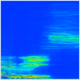
FFT is a perfect tool to record the spectral behavior of a sound varying in time, such as a spoken word. Of course in this case, the signal is no longer periodical, but you can assume that it is somewhat periodic piecewise. That is why FFT is often used for short signal blocks, for example for a block length of 100 ms, and repeated every 2.5 ms. Hence, we get a new spectrum for every 2.5 ms that can be represented as a colored vertical line in a sonogram.
from soundsystem import * from gpanel import * def toColor(z): w = int(450 + 300 * z) c = X11Color.wavelengthToColor(w) return c def drawSonogram(): makeGPanel(0, 190, 0, 1000) title("Sonogramm of 'Harris'") lineWidth(4) # Analyse blocks every 50 samples for k in range(191): a = fft(samples[k * 50:], n) for i in range(n // 2): setColor(toColor(a[i])) point(k, i) fs = 20000 # Sampling freq->spectrum 0..10 kHz n = 2000 # Size of block for analyser samples = getWavMono("wav/harris.wav") openMonoPlayer(samples, fs) play() drawSonogram() |
MEMO |
The sonogram shows frequencies in the range from 0..10 kHz vertically, and the course of time from 0 to 190 * 50 / 20000 = 0.475 s horizontally. To convert numbers to colors, you should use the function X11Color.wavelengthToColor() which converts the wavelengths of the color spectrum to colors in the range 380...780 nm. The high spectral components for the sibilant "s" are clearly visible, whereas the fundamentals are entirely missing. |
LIGHT SPECTRA |
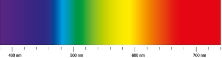
Light can also be decomposed spectrally in order to determine its contained wavelength components. The wavelengths of the visible spectrum ranges from about 380 nm to 780 nm.
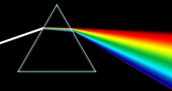
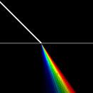
It is quite likely that you already know the spectrum analyzer for light, called a prism, which refracts (breaks up) light of various wavelengths at different angles according to the law of refraction.
In your program, you simulate the transition of a white beam of light in glass and show in a magnification the paths of the different colors. from gpanel import * # K5 glass B = 1.5220 C = 4590 # nanometer^2 # Cauchy equation for refracting index def n(wavelength): return B + C / (wavelength * wavelength) makeGPanel(-1, 1, -1, 1) title("Refracting at the K5 glass") bgColor("black") setColor("white") line(-1, 0, 1, 0) lineWidth(4) line(-1, 1, 0, 0) lineWidth(1) sineAlpha = 0.707 for i in range(51): wavelength = 380 + 8 * i setColor(X11Color.wavelengthToColor(wavelength)) sineBeta = sineAlpha / n(wavelength) x = (sineBeta - 0.45) * 100 - 0.5 # magnification line(0, 0, x, -1) |
MEMO |
If you want to create a beautiful graphic, you should refract the colors more than they would be in real life. |
EXERCISES |
|