8.6 CORRELATION, REGRESSION
![]()
INTRODUCTION |
In both the natural sciences and in daily life, the collection of data in the form of measurements plays an important role. However, you do not always need to use a measuring instrument. The data can also consist in poll values, for example, in connection with a statistical investigation. After any data acquisition, it is most important to interpret the measured data. You may look for qualitative statements where the measured values rise or fall over time, or you might want experimentally verify a law of nature. A major problem is that measurements are almost always subject to fluctuations and are not exactly reproducible. Despite these "measurement errors" people would still like to make scientifically correct statements. Measurement errors do not always emerge from flawed measuring instruments, but they may also lie in the nature of the experiment. For instance, the "measurement" of the numbers on a rolled die basically results in dispersed values between 1 and 6. Therefore, with any type of measurement, statistical considerations play a central role. Often two variables x and y are measured together in a measurement series and questions arise as to whether these are related and if they are subject to regularity. Plotting the (x, y) values as measuring points in a coordinate system is called data visualization. You can almost always recognize whether the data are dependent of each other by simply looking at the distribution of the measured values.
|
VISUALIZING INDEPENDENT AND DEPENDENT DATA |
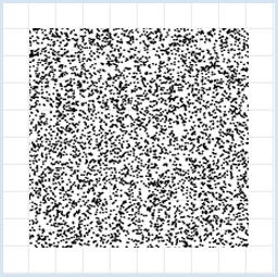
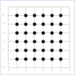
from random import random
from gpanel import *

z = 10000

makeGPanel(-1, 11, -1, 11)
title("Uuniformly distributed value pairs")
drawGrid(10, 10, "gray")

xval = [0] * z
yval = [0] * z

for i in range(z):
    xval[i] = 10 * random()
    yval[i] = 10 * random()
    move(xval[i], yval[i])
    fillCircle(0.03)
Highlight program code
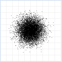
from random import gauss
from gpanel import *

z = 10000

makeGPanel(-1, 11, -1, 11)
title("Normally distributed value pairs")
drawGrid(10, 10, "gray")

xval = [0] * z
yval = [0] * z

for i in range(z):
    xval[i] = gauss(5, 1)
    yval[i] = gauss(5, 1)
    move(xval[i], yval[i])
    fillCircle(0.03)
Highlight program code
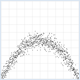
from random import gauss
from gpanel import *
import math

z = 1000
a = 0.2
b = 2

def f(x):
    y = -x * (a * x - b)
    return y

makeGPanel(-1, 11, -1, 11)
title("y = -x * (0.2 * x - 2) with normally distributed noise")
drawGrid(0, 10, 0, 10, "gray")

xval = [0] * z
yval = [0] * z

for i in range(z):
    x = i / 100
    xval[i] = x
    yval[i] = f(x) + gauss(0, 0.5)
    move(xval[i], yval[i])
    fillCircle(0.03)
Highlight program code
|
MEMO |
|
You can recognize interdependencies of measured variables immediately through the use of data visualization [more... This example is characterized famous because correlation does not recognize the dependence]. With uniformly distributed random numbers in an interval [a, b], the numbers appear with the same frequency in each subinterval of equal length. Normally distributed numbers have a bell-shape distribution, where 68% of the numbers lie inside the interval (average - dispersion) and (average + dispersion). |
COVARIANCE AS A MEASURE FOR DEPENDENCY |
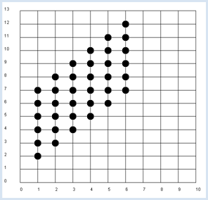
Since x and y are independent, the probability pxy, to get the pair x, y from a double roll is pxy = px * py. It is an obvious assumption that in the general case the following product rule applies. If x and y are independent, the expected value of x * y equals the product of the expected values of x and y [more... The theoretical proof is simple:] . This assumption is confirmed in the simulation. from random import randint from gpanel import * z = 10000 # number of double rolls def dec2(x): return str(round(x, 2)) def mean(xval): n = len(xval) count = 0 for i in range(n): count += xval[i] return count / n makeGPanel(-1, 8, -1, 8) title("Double rolls. Independent random variables") addStatusBar(30) drawGrid(0, 7, 0, 7, 7, 7, "gray") xval = [0] * z yval = [0] * z xyval = [0] * z for i in range(z): a = randint(1, 6) b = randint(1, 6) xval[i] = a yval[i] = b xyval[i] = xval[i] * yval[i] move(xval[i], yval[i]) fillCircle(0.2) xm = mean(xval) ym = mean(yval) xym = mean(xyval) setStatusText("E(x) = " + dec2(xm) + \ ", E(y) = " + dec2(ym) + \ ", E(x, y) = " + dec2(xym)) Highlight program code
|
MEMO |
|
It is advisable to use a status bar where the results can be written out. The function dec2() rounds the value to 2 digits and returns it as a string. The values are of course subject to a statistical fluctuation. In the next simulation you will no longer analyze the rolled pair of numbers, but rather the numbers x of the first die and the sum y of the two rolled numbers. It is now evident that y is dependent on x, for example if x = 1, the probability of y = 4 is not the same as when x = 2. |
from random import randint
from gpanel import *

z = 10000 # number of double rolls

def dec2(x):
    return str(round(x, 2))

def mean(xval):
    n = len(xval)
    count = 0
    for i in range(n):
        count += xval[i]
    return count / n

def covariance(xval, yval):
    n = len(xval)
    xm = mean(xval)
    ym = mean(yval)
    cxy = 0
    for i in range(n):
       cxy += (xval[i] - xm) * (yval[i] - ym)
    return cxy / n

makeGPanel(-1, 11, -2, 14)
title("Double rolls. Independent random variables")
addStatusBar(30)
drawGrid(0, 10, 0, 13, 10, 13, "gray")

xval =  [0] * z
yval =  [0] * z
xyval = [0] * z

for i in range(z):
    a = randint(1, 6)
    b = randint(1, 6)
    xval[i] = a
    yval[i] = a + b
    xyval[i] = xval[i] * yval[i]
    move(xval[i], yval[i])
    fillCircle(0.2)

xm = mean(xval)
ym = mean(yval)
xym = mean(xyval)
c = xym - xm * ym
setStatusText("E(x) = " + dec2(xm) + \
          ",  E(y) = " + dec2(ym) + \
          ",  E(x, y) = " + dec2(xym) + \
          ",  c = " + dec2(c) + \
          ",  covariance = " + dec2(covariance(xval, yval)))
Highlight program code
|
MEMO |
|
You get a value of about 2.9 for the covariance in the simulation. The covariance is therefore well qualified as a measure for the dependence of random variables. |
THE CORRELATION COEFFICIENT |
The just introduced covariance also has a disadvantage. Depending on how the measured values x and y are scaled, different values occur, even if the values are apparently equally dependent on each other. This is easy to see. If you take, for example, two dice that have sides with numbers going from 10 to 60 instead of from 1 to 6, the covariance changes greatly even though the dependence is the same. This is why you introduce a normalized covariance, called a correlation coefficient, by dividing the covariance by the dispersion of the x and y values
The correlation coefficient is always in the range from -1 to 1. A value close to 0 corresponds to a small dependence and a value close to 1 represents a large dependence, whereas increasing values of x correspond to increasing values of y, and a value close to -1 corresponds to increasing values of x and decreasing values of y. You again use the double roll in the program and analyze the dependence of the sum of the numbers from the number of the first die. from random import randint from gpanel import * import math z = 10000 # number of double rolls k = 10 # scalefactor def dec2(x): return str(round(x, 2)) def mean(xval): n = len(xval) count = 0 for i in range(n): count += xval[i] return count / n def covariance(xval, yval): n = len(xval) xm = mean(xval) ym = mean(yval) cxy = 0 for i in range(n): cxy += (xval[i] - xm) * (yval[i] - ym) return cxy / n def deviation(xval): n = len(xval) xm = mean(xval) sx = 0 for i in range(n): sx += (xval[i] - xm) * (xval[i] - xm) sx = math.sqrt(sx / n) return sx def correlation(xval, yval): return covariance(xval, yval) / (deviation(xval) * deviation(yval)) makeGPanel(-1 * k, 11 * k, -2 * k, 14 * k) title("Double rolls. Independent random variables.") addStatusBar(30) drawGrid(0, 10 * k, 0, 13 * k, 10, 13, "gray") xval = [0] * z yval = [0] * z xyval = [0] * z for i in range(z): a = k * randint(1, 6) b = k * randint(1, 6) xval[i] = a yval[i] = a + b xyval[i] = xval[i] * yval[i] move(xval[i], yval[i]) fillCircle(0.2 * k) xm = mean(xval) ym = mean(yval) xym = mean(xyval) c = xym - xm * ym setStatusText("E(x) = " + dec2(xm) + \ ", E(y) = " + dec2(ym) + \ ", E(x, y) = " + dec2(xym) + \ ", covariance = " + dec2(covariance(xval, yval)) + \ ", correlation = " + dec2(correlation(xval, yval))) Highlight program code
|
MEMO |
|
You can change the scaling factor k and the correlation will stay around 0.71, as opposed to the covariance which greatly changes [more...
The correlation coefficient checks only linear dependencies. Instead of always calling it the correlation coefficient, you can simply call it correlation. |
MEDICAL RESEARCH PUBLICATION |
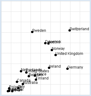
Nobel Prizes: Chocolate consumption: You want to reconstruct the investigation yourself. In your program, you use a list data with sub-lists of three elements: the name of the country, the amount of chocolate consumption in kg per year and per inhabitant, and the number of Nobel Prize winners per 10 million inhabitants. You display the data graphically and determine the correlation coefficient. from gpanel import * import math data = [["Australia", 4.8, 5.141], ["Austria", 8.7, 24.720], ["Belgium", 5.7, 9.005], ["Canada", 3.9, 6.253], ["Denmark", 8.2, 24.915], ["Finland", 6.8, 7.371], ["France", 6.6, 9.177], ["Germany", 11.6, 12.572], ["Greece", 2.5, 1.797], ["Italy", 4.1, 3.279], ["Ireland", 8.8, 12.967], ["Netherlands", 4.5, 11.337], ["Norway", 9.2, 21.614], ["Poland", 2.7, 3.140], ["Portugal", 2.7, 1.885], ["Spain", 3.2, 1.705], ["Sweden", 6.2, 30.300], ["Switzerland", 11.9, 30.949], ["United Kingdom", 9.8, 19.165], ["United States", 5.3, 10.811]] def dec2(x): return str(round(x, 2)) def mean(xval): n = len(xval) count = 0 for i in range(n): count += xval[i] return count / n def covariance(xval, yval): n = len(xval) xm = mean(xval) ym = mean(yval) cxy = 0 for i in range(n): cxy += (xval[i] - xm) * (yval[i] - ym) return cxy / n def deviation(xval): n = len(xval) xm = mean(xval) sx = 0 for i in range(n): sx += (xval[i] - xm) * (xval[i] - xm) sx = math.sqrt(sx / n) return sx def correlation(xval, yval): return covariance(xval, yval) / (deviation(xval) * deviation(yval)) makeGPanel(-2, 17, -5, 55) drawGrid(0, 15, 0, 50, "lightgray") xval = [] yval = [] for country in data: d = country[1] v = country[2] xval.append(d) yval.append(v) move(d, v) fillCircle(0.2) text(country[0]) title("Chocolate-Brainpower-Correlation: " + dec2(correlation(xval, yval))) Highlight program code
|
MEMO |
|
This results in a high correlation of approximately 0.71, which can be interpreted in different ways. It is right to say that there is a correlation between the two sets of data, but we can only speculate about the reasons why. In particular a causal relationship between the consumption of chocolate and intelligence can by no means be proven this way. As a general rule: When there is a high correlation between x and y, x can be the cause for the behavior of y. Likewise, y can be the cause for the behavior of x, or x and y can be associated with other perhaps unknown causes. Discuss the meaning and purpose of this investigation with other people in your community and ask them for their opinion. |
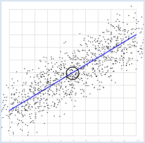
MEASUREMENT ERRORS AND NOISE |
from random import gauss
from gpanel import *
import math

z = 1000
a = 0.6
b = 2
sigma = 1

def f(x):
    y = a * x + b
    return y

def dec2(x):
    return str(round(x, 2))

def mean(xval):
    n = len(xval)
    count = 0
    for i in range(n):
        count += xval[i]
    return count / n

def covariance(xval, yval):
    n = len(xval)
    xm = mean(xval)
    ym = mean(yval)
    cxy = 0
    for i in range(n):
       cxy += (xval[i] - xm) * (yval[i] - ym)
    return cxy / n

def deviation(xval):
    n = len(xval)
    xm = mean(xval)
    sx = 0
    for i in range(n):
        sx += (xval[i] - xm) * (xval[i] - xm)
    sx = math.sqrt(sx / n)
    return sx

def correlation(xval, yval):
    return covariance(xval, yval) / (deviation(xval) * deviation(yval))

makeGPanel(-1, 11, -1, 11)
title("y = 0.6 * x + 2 normally distributed measurement errors")
addStatusBar(30)
drawGrid(0, 10, 0, 10, "gray")
setColor("blue")
lineWidth(3)
line(0, f(0), 10, f(10))

xval = [0] * z
yval = [0] * z

setColor("black")
for i in range(z):
    x = i / 100
    xval[i] = x
    yval[i] = f(x) + gauss(0, sigma)
    move(xval[i], yval[i])
    fillCircle(0.03)

xm = mean(xval)
ym = mean(yval)
move(xm, ym)
circle(0.5)

setStatusText("E(x) = " + dec2(xm) + \
          ",  E(y) = " + dec2(ym) + \
          ",  correlation = " + dec2(correlation(xval, yval)))
Highlight program code
|
MEMO |
|
This results in a high correlation as expected, which becomes even greater the smaller the selected dispersion sigma is. The correlation is exactly 1 for sigma = 0. |
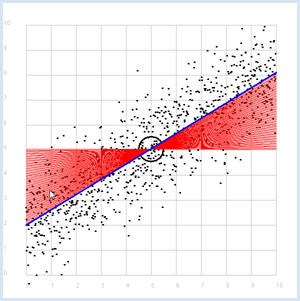
REGRESSION LINE, BEST FIT |
Previously you started with a straight line, that you made "noisy" yourself. Here, you ask the opposite question: How do you detect the straight line again if you only have the two series of measurements? The desired line is called the regression line. At least you already know that the regression line passes through the point P with the expected values. To find it, you can do the following:
from random import gauss
from gpanel import *
import math

z = 1000
a = 0.6
b = 2

def f(x):
    y = a * x + b
    return y

def dec2(x):
    return str(round(x, 2))

def mean(xval):
    n = len(xval)
    count = 0
    for i in range(n):
        count += xval[i]
    return count / n

def covariance(xval, yval):
    n = len(xval)
    xm = mean(xval)
    ym = mean(yval)
    cxy = 0
    for i in range(n):
       cxy += (xval[i] - xm) * (yval[i] - ym)
    return cxy / n

def deviation(xval):
    n = len(xval)
    xm = mean(xval)
    sx = 0
    for i in range(n):
        sx += (xval[i] - xm) * (xval[i] - xm)
    sx = math.sqrt(sx / n)
    return sx

sigma = 1

makeGPanel(-1, 11, -1, 11)
title("Simulate data points. Press a key...")
addStatusBar(30)
drawGrid(0, 10, 0, 10, "gray")
setStatusText("Press any key")

xval = [0] * z
yval = [0] * z

for i in range(z):
    x = i / 100
    xval[i] = x
    yval[i] = f(x) + gauss(0, sigma)
    move(xval[i], yval[i])
    fillCircle(0.03)

getKeyWait()
xm = mean(xval)
ym = mean(yval)
move(xm, ym)
lineWidth(3)
circle(0.5)

def g(x):
    y = m * (x - xm) + ym
    return y

def errorSum():
    count = 0
    for i in range(z):
        x = i / 100
        count += (yval[i] - g(x)) * (yval[i] - g(x))
    return count

m = 0
setColor("red")
lineWidth(1)
error_min = 0
while m < 5:
    line(0, g(0), 10, g(10))
    if m == 0:
        error_min = errorSum()
    else:
        if errorSum() < error_min:
            error_min = errorSum()
        else:
            break
    m += 0.01

title("Regression line found")
setColor("blue")
lineWidth(3)
line(0, g(0), 10, g(10))
setStatusText("Found slope: " +  dec2(m) + \
               ", Theory: " + dec2(covariance(xval, yval)
              /(deviation(xval) * deviation(xval))))
Highlight program code
|
MEMO |
|
Instead of using a computer simulation to find the best fit, you can also directly calculate the slope of the regression line.
Since the line passes through the point P with the expected values E(x) and E(y), it thus has the linear equation:
|
EXERCISES |
|
ADDITIONAL MATERIAL |
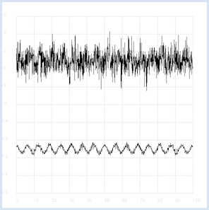
FINDING CACHED INFORMATION WITH AUTOCORRELATION |
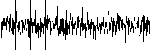
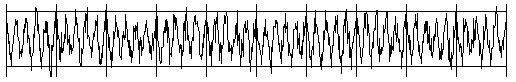
Intelligent beings on a distant planet want to contact other living beings. To do this, they send out radio signals that present a certain regularity (you can imagine a kind of Morse code). The signal becomes weaker and weaker on the long transmission path and gets masked by statistically fluctuating noise. We receive this signal on Earth with a radio telescope, and so for the time being we only hear the noise. The statistics and a computer program can help us retrieve the original radio signal again. If you calculate the correlation coefficient of the signal with its own time-shifted signal, you decrease the statistical noise components. (A correlation with itself is called an autocorrelation).
from random import gauss
from gpanel import *
import math

def mean(xval):
    n = len(xval)
    count = 0
    for i in range(n):
        count += xval[i]
    return count / n

def covariance(xval, yval):
    n = len(xval)
    xm = mean(xval)
    ym = mean(yval)
    cxy = 0
    for i in range(n):
       cxy += (xval[i] - xm) * (yval[i] - ym)
    return cxy / n

def deviation(xval):
    n = len(xval)
    xm = mean(xval)
    sx = 0
    for i in range(n):
        sx += (xval[i] - xm) * (xval[i] - xm)
    sx = math.sqrt(sx / n)
    return sx

def correlation(xval, yval):
    return covariance(xval, yval)/(deviation(xval)*deviation(yval))
def shift(offset):
    signal1 = [0] * 1000
    for i in range(1000):
       signal1[i] = signal[(i + offset) % 1000]
    return signal1

makeGPanel(-10, 110, -2.4, 2.4)
title("Noisy signal. Press a key...")
drawGrid(0, 100, -2, 2.0, "lightgray")

t = 0
dt = 0.1
signal = [0] * 1000
while t < 100:
    y = 0.1 * math.sin(t) # Pure signal
#    noise = 0
    noise = gauss(0, 0.2)
    z = y + noise
    if t == 0:
        move(t, z + 1)
    else:
        draw(t, z + 1)
    signal[int(10 * t)] = z
    t += dt

getKeyWait()
title("Signal after autocorrelation")
for di in range(1, 1000):
    y = correlation(signal, shift(di))
    if di == 1:
        move(di / 10, y - 1)
    else:
        draw(di / 10, y - 1)
Highlight program code
To make it a bit more exciting, listen to the noisy signal first and then the extracted useful signal. To do this, tap into your knowledge from the chapter on Sound. from soundsystem import * import math from random import gauss from gpanel import * n = 5000 def mean(xval): count = 0 for i in range(n): count += xval[i] return count / n def covariance(xval, k): cxy = 0 for i in range(n): cxy += (xval[i] - xm) * (xval[(i + k) % n] - xm) return cxy / n def deviation(xval): xm = mean(xval) sx = 0 for i in range(n): sx += (xval[i] - xm) * (xval[i] - xm) sx = math.sqrt(sx / n) return sx makeGPanel(-100, 1100, -11000, 11000) drawGrid(0, 1000, -10000, 10000) title("Press <SPACE> to repeat. Any other key to continue.") signal = [] for i in range(5000): value = int(200 * (math.sin(6.28 / 20 * i) + gauss(0, 4))) signal.append(value) if i == 0: move(i, value + 5000) elif i <= 1000: draw(i, value + 5000) ch = 32 while ch == 32: openMonoPlayer(signal, 5000) play() ch = getKeyCodeWait() title("Autocorrelation running. Please wait...") signal1 = [] xm = mean(signal) sigma = deviation(signal) q = 20000 / (sigma * sigma) for di in range(1, 5000): value = int(q * covariance(signal, di)) signal1.append(value) title("Autocorrelation Done. Press any key to repeat.") for i in range(1, 1000): if i == 1: move(i, signal1[i] - 5000) else: draw(i, signal1[i] - 5000) while True: openMonoPlayer(signal1, 5000) play() getKeyCodeWait() Highlight program code
|
MEMO |
|
Instead of executing the program, you can listen to the two signals as WAV files here Noisy signal (click here)
Desired signal (click here)
|