8.4 AVERAGE WAITING TIMES
![]()
INTRODUCTION |
|
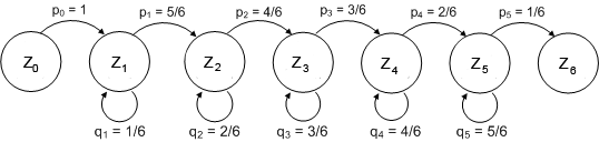
There are many systems whose temporal behavior can be described as transitions from one state to the next. The transition from a current system state Zito the following state Zkis determined by probabilities pik. In the example below, you will roll one die and consider the already rolled numbers as a state variables: Z0 : no number rolled yet You can illustrate the transition of the states as in the scheme below (called Markov chain):
The probabilities are understood as follows: if you have already rolled n numbers, the chances of getting one of these numbers again is n/6 and the chance of getting a number you have not yet rolled is (6 - n)/6. You can attempt to solve the interesting question of how many times you have to roll the die on average to get all six numbers.
|
AVERAGE WAITING TIMES |
If you roll the die in equal increments of time, you can also ask yourself how long, on average, the process takes. You call this time the average waiting time. You can figure it out with the following reflection: the total time to get from Z0 to Z6is the sum of the waiting times for all transitions. But how long are the individual waiting times? In your first program you can experimentally determine the most important feature of waiting time problems: If p is the probability of getting from Z1 to Z2the delay time amounts to (in a suitable unit) u = 1/p.
from gpanel import * from random import randint n = 10000 p = 1/6 def sim(): k = 1 r = randint(1, 6) while r != 6: r = randint(1, 6) k += 1 return k makeGPanel(-5, 55, -200, 2200) drawGrid(0, 50, 0, 2000) title("Waiting on a 6") h = [0] * 51 lineWidth(5) count = 0 repeat n: k = sim() count += k if k <= 50: h[k] += 1 line(k, 0, k, h[k]) mean_exp = count / n lineWidth(1) setColor("red") count = 0 for k in range(1, 1000): pk = (1 - p)**(k - 1) * p nk = n * pk count += nk * k if k <=50: line(k, 0, k, nk) mean_theory = count / n title("Experiment: " + str(mean_exp) + "Theory: " + str(mean_theory)) |
MEMO |
|
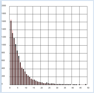
The result is intuitively evident: since the probability of rolling a certain number on the die is p= 1/6, you need an average of u = 1 / p = 6 rolls to get this number. It is also instructive to display the theoretical values of the frequencies as a red line. To do this, you must consider that the following applies to the probability of rolling a 6:
To get the theoretical frequencies, multiply these probabilities with the number of trials n [more... With a little algebra one can prove that the expected value of the Waiting time = sum of pk * k is actually exactly 1/p ]. |
PROGRAMMING INSTEAD OF A LOT OF CALCULATING |
In order to solve the task defined above, to calculate the average delay until you have rolled all numbers at least once, you may decide to take the theoretical path. You interpret the process as a Markov chain and add the delay times of each individual transition: u = 1 + 6/5 + 6/4 + 6/3 + 6/2 + 6 = 14.7 Alternatively, you can write a simple program to determine this number in a simulation. To do this, you always proceed the same way: write a function sim() where the computer searches for a single solution using random numbers and then returns the required number of steps as a return value. You then repeat this task many times, let's say 1,000 times, and determine the average value. It is smart to use a list z in sim(), where you can insert the rolled numbers that are not already there. Once the list has 6 elements, you have rolled all the numbers of the die. from random import randint n = 10000 def sim(): z = [] i = 0 while True: r = randint(1, 6) i += 1 if not r in z: z.append(r) if len(z) == 6: return i count = 0 repeat n: count += sim() print("Mean waiting time:", count / n) |
MEMO |
In the computer simulation you get the slightly fluctuating value 14.68, which corresponds to the theoretical prediction. The computer can thus also be used to quickly check if a theoretically calculated value can be correct.
However, the theoretical determination of waiting times can already be very complex with simple problems. If you are, for instance, trying to figure out the average waiting time until you have rolled a certain sum of numbers, the problem is extremely easy to solve with a computer simulation from random import randint n = 10000 s = 7 # rolled count of the die numbers def sim(): i = 0 total = 0 while True: i += 1 r = randint(1, 6) total += r if total >= s: break return i count = 0 repeat n: count += sim() print("Mean waiting time:", count / n) |
MEMO |
You get an average delay time of about 2.52 for rolling the sum 7 with the die. This result is somewhat surprising, given that the expected value for the die numbers is 3.5. Therefore, it could be assumed that you have to roll the die 2x on average to achieve the sum 7. |
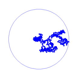
THE SPREADING OF AN DISEASE |
Assume the following story. Even though it is fictional, there are certain parallels to current living communities.
It is smart to model the population with a list with Boolean values, where healthy is coded as False and ill as True. The advantage of this data structure is that in the function pair(), the interaction that occurs when two people meet can simply be expressed by a logical OR operation:
from gpanel import * from random import randint def pair(): # Select two distinct inhabitants a = randint(0, 99) b = a while b == a: b = randint(0, 99) z[a] = z[a] or z[b] z[b] = z[a] def nbInfected(): count = 0 for i in range(100): if z[i]: count += 1 return count makeGPanel(-50, 550, -10, 110) title("The spread of an illness") drawGrid(0, 500, 0, 100) lineWidth(2) setColor("blue") z = [False] * 100 tmax = 500 t = 0 a = randint(0, 99) z[a] = True # random infected inhabitant move(t, 1) while t <= tmax: pair() infects = nbInfected() t += 1 draw(t, infects) |
MEMO |
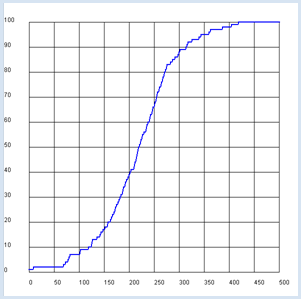
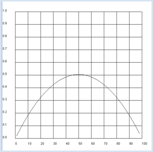
You will find a temporal behavior where the increase is first slow, then rapid, and then slow again. This behavior is certainly feasible qualitatively since the probability is at first low that an ill person encounters a healthy person, since mostly healthy people meet each other. At the end the probability is again low that a remaining healthy person encounters an ill person, since mainly sick people are meeting each other [more... The curve corresponds to the logistic growth]. |
from random import randint n = 1000 # number experiment def pair(): # Select two distinct inhabitants a = randint(0, 99) b = a while b == a: b = randint(0, 99) z[a] = z[a] or z[b] z[b] = z[a] def nbInfected(): count = 0 for i in range(100): if z[i]: count += 1 return count def sim(): global z z = [False] * 100 t = 0 a = randint(0, 99) z[a] = True # random infected inhabitant while True: pair() t += 1 if nbInfected() == 100: return t count = 0 for i in range(n): u = sim() print("Experiment #", i + 1, "Waiting time:", u) count += u print( "Mean waiting time:", count / n) You can also illustrate the spread of the disease as a Markov chain. A certain state is characterized by the number of people infected. The time until everyone is ill is the sum of the waiting time for the transitions from k ill people to k+1 ill people, for k from 1 to 99. In addition, you need the probability pkfor this transition. It is:
from gpanel import * n = 100 def p(k): return 2 * k * (n - k) / n / (n - 1) makeGPanel(-10, 110, -0.1, 1.1) drawGrid(0, 100, 0, 1.0) count = 0 for k in range(1, n - 1): if k == 1: move(k, p(k)) else: draw(k, p(k)) count += 1 / p(k) title("Time until everyone is ill: " + str(count)) |
MEMO |
Using the theory of Markov chains results in an average waiting time of 463 hours until everyone has the illness, or around 20 days. |
PARTNER SEARCHING WITH A PROGRAM |
An interesting matter for practice is the optimal strategy in the selection of a life partner. In this case you start based on the following model assumption: 100 potential partners possess increasing qualification levels. They will be presented to you in a random order and in a "learning phase" you can correctly order them by qualification levels, by relying on your previous life experiences. However, you do not know what the maximum degree of qualification is. With each introduction, you have to decide if you want to accept or reject the partner. What should you do to make sure that you choose the partner with the best qualifications with a high probability? For the simulation, create a list t with the 100 qualification levels from 0 to 99 in any order in the function sim(x). It consists of a random permutation of the numbers 0 to 99, that you can nicely create in Python with shuffle().
from random import shuffle
from gpanel import *

n = 1000 # Number of simulations
a = 100 # Number of partners

def sim(x):
    # Random permutation [0..99]
    t = [0] * 100
    for i in range(0, 100):
        t[i] = i
    shuffle(t)
    best = max(t[0:x])
    for i in range(x, 100):
        if  t[i] > best:
            return [i, t[i]]
    return [99, t[99]]

makeGPanel(-10, 110, -0.1, 1.1)
title("The probability of finding the best partner from  100")
drawGrid(0, 100, 0, 1.0)

for x in range(1, 100):
    count = 0
    repeat n:
        z = sim(x)
        if z[1] == 99:  # best score
            count += 1
    p = count / n
    if x == 1:
        move(x, p)
    else:
        draw(x, p)
|
MEMO |
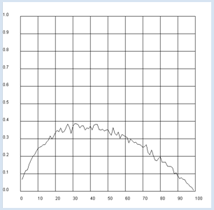
Apparently you are the likeliest to find the partner with the best qualifications after a learning phase of around 37 [more... The theoretical value is 100 / e]. |
from random import shuffle from gpanel import * n = 1000 # Number of simulations def sim(x): # Random permutation [0..99] t = [0] * 100 for i in range(0, 100): t[i] = i shuffle(t) best = max(t[0:x]) for i in range(x, 100): if t[i] > best: return [i, t[i]] return [99, t[99]] makeGPanel(-10, 110, -10, 110) title("Mean qualification after waiting for a partner") drawGrid(0, 100, 0, 100) for x in range(1, 99): count = 0 repeat n: u = sim(x) count += u[1] y = count / n if x == 1: move(x, y) else: draw(x, y) |
MEMO |
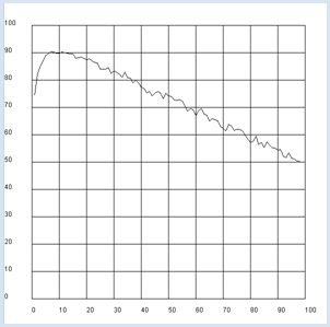
This looks entirely different: following the criterion of the best possible average qualification, you should already make your decision for the next better rated partner after a learning phase of about 10 . You can also perform the simulation for a more realistic number of partners and notice that the optimal learning phase is quite short [more...However, the maximum achievable medium level decreases with a smaller selection] |
WAITING TIME PARADOX |
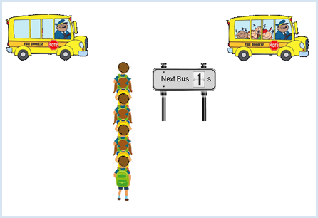
Since they still come by every 6 minutes on average in this case, it is possible that you assume that the waiting time of 3 minutes stays the same. The surprising and therefore paradoxical answer is that the average waiting time is greater than 3 minutes in this situation. In an animated simulation you should find out how long the waiting time is under the assumption that the buses are uniformly distributed to arrive one after another between every 2 to 10 minutes (in the simulation these are seconds). You can use the game library JGameGrid for this since you can easily model objects such as buses and passengers as sprite objects.
The program code requires some explanation: Since we are obviously dealing with bus and passenger objects, they are modeled by the classes Bus and Passenger. The buses are created in an infinite loop at the end of the main part of the program according to the statistical requirements. When the graphics window is closed the infinite loop breaks due to isDisposed() = False and the program ends. The passengers must be periodically generated and displayed in the queue. The best way to do this, is to write a class PassengerFactory that is derived from Actor. Even though this does not have a sprite image, its act() can be used to generate passengers and to insert them into the GameGrid. You can select the period at which the objects are generated using the cycle counter nbCycles (the simulation cycle is set to 50 ms). You move the bus forward in the act() of the class Bus and check if it has arrived at the stop with the x-coordinate. When it arrives, you call the method board() of the class PassengerFactory whereby the waiting passengers are removed from the queue. Simultaneously change the sprite image of the buses with show(1) and show the new waiting time for the next bus on the scoreboard. Use the Boolean variable isBoarded so that these actions are only called once. The scoreboard as an instance of the class InformationPanel is an additional gadget to show the time it will take until the next bus arrives. The display will again be changed in the method act() by selecting one of the 10 sprite images (digit_0.png to digit_9.png) using show(). from gamegrid import * from random import random, randint import time min_value = 2 max_value = 10 def random_t(): return min_value + (max_value - min_value) * random() # ---------------- class PassengerFactory ---------- class PassengerFactory(Actor): def __init__(self): self.nbPassenger = 0 def board(self): for passenger in getActors(Passenger): passenger.removeSelf() passenger.board() self.nbPassenger = 0 def act(self): if self.nbCycles % 10 == 0: passenger = Passenger( randint(0, 1)) addActor(passenger, Location(400, 120 + 27 * self.nbPassenger)) self.nbPassenger += 1 # ---------------- class Passenger ----------------- class Passenger(Actor): totalTime = 0 totalNumber = 0 def __init__(self, i): Actor.__init__(self, "sprites/pupil_" + str(i) + ".png") self.createTime = time.clock() def board(self): self.waitTime = time.clock() - self.createTime Passenger.totalTime += self.waitTime Passenger.totalNumber += 1 mean = Passenger.totalTime / Passenger.totalNumber setStatusText("Mean waiting time: " + str(round(mean, 2)) + " s") # ---------------- class Car ----------------------- class Bus(Actor): def __init__(self, lag): Actor.__init__(self, "sprites/car1.gif") self.lag = lag self.isBoarded = False def act(self): self.move() if self.getX() > 320 and not self.isBoarded: passengerFactory.board() self.isBoarded = True infoPanel.setWaitingTime(self.lag) if self.getX() > 1650: self.removeSelf() # ---------------- class InformationPanel ---------- class InformationPanel(Actor): def __init__(self, waitingTime): Actor.__init__(self, "sprites/digit.png", 10) self.waitingTime = waitingTime def setWaitingTime(self, waitingTime): self.waitingTime = waitingTime def act(self): self.show(int(self.waitingTime + 0.5)) if self.waitingTime > 0: self.waitingTime -= 0.1 periodic = askYesNo("Departures every 6 s?") makeGameGrid(800, 600, 1, None, None, False) addStatusBar(20) setStatusText("Acquiring data...") setBgColor(Color.white) setSimulationPeriod(50) show() doRun() if periodic: setTitle("Warting Time Paradoxon - Departure every 6 s") else: setTitle("Waiting Time Paradoxon - Departure between 2 s and 10 s") passengerFactory = PassengerFactory() addActor(passengerFactory, Location(0, 0)) addActor(Actor("sprites/panel.png"), Location(500, 120)) addActor(TextActor("Next Bus"), Location(460, 110)) addActor(TextActor("s"), Location(540, 110)) infoPanel = InformationPanel(4) infoPanel.setSlowDown(2) addActor(infoPanel, Location(525, 110)) while not isDisposed(): if periodic: lag = 6 else: lag = random_t() bus = Bus(lag) addActor(bus, Location(-100, 40)) a = time.clock() while time.clock() - a < lag and not isDisposed(): delay(10)
|

MEMO |
The simulation shows that the average waiting time is around 3.5 minutes, so in other words clearly longer than the previously assumed 3 minutes. You can explain this change as follows: If the buses arrive equally distributed, once with a gap of 2 minutes and once with a gap of 10 minutes, it is much more likely that you will get to the bus stop during the waiting interval from 2 to 10 minutes, rather than 0 to 2 minutes. Therefore, you will certainly end up waiting longer than 3 minutes. |
EXERCISES |
|