3.10 RANDOMNESS
![]()
INTRODUCTION |
|
Chance plays an important role in your daily life. We can think of it as events that are not predictable. If you are asked to choose from the colors red, green, and blue, no one can predict which one you will choose and therefore the color is random. Chance plays a big role in games as well: If you roll a dice, the number of pips you get, between 1 and 6, is random. Although the world is ruled by chance it is not chaotic, since even in chance there are regularities that allow for certain predictions. However, these only apply "on average", or in other words, if you are in the same situation many times. In order to investigate the laws of chance, you must make random experiments where you define the specific initial conditions, but where the process is controlled by random numbers. The computer is exceptionally well suited for random experiments because it is easy to perform a large number of experiments. For this, the computer must generate a series of random numbers that are independent of each other. You most often use integers with a certain predetermined range, e.g. between 1 and 6, or a decimal number between 0 and 1. An algorithm that computes a set of random numbers is called a random number generator. It is important that the numbers occur with the same frequency as you would expect from a non-marked dice. We call such numbers uniformly distributed . |
RANDOM PAINTING |
from gpanel import * from random import randint, random def randomColor(): r = randint(0, 255) g = randint(0, 255) b = randint(0, 255) return makeColor(r, g, b) makeGPanel() bgColor(randomColor()) for i in range(20): setColor(randomColor()) move(random(), random()) a = random() / 2 b = random() / 2 fillEllipse(a, b) |

MEMO |
|
random() returns uniformly distributed random numbers as floats between 0 (included) and 1 (excluded). You have to import the random module in order to access it. Colors are defined by their red, green, and blue parts (RGB). The values are integers between 0 and 255. Using randint(start, end) you get a random integer between start and end (both included). The function makeColor() returns a color object from 3 color values for red, green, and blue. |
FREQUENCY OF DICE NUMBERS |
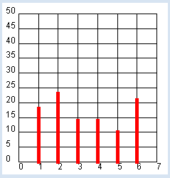
from gpanel import * from random import randint NB_ROLLS = 100 makeGPanel(-1, 8, -0.1 * NB_ROLLS / 2, 1.1 * NB_ROLLS / 2) title("# Rolls: " + str(NB_ROLLS)) drawGrid(0, 7, 0, NB_ROLLS // 2, 7, 10) setColor("red") histo = [0, 0, 0, 0, 0, 0, 0] # hist = [0] * 7 # short form for i in range(NB_ROLLS): pip = randint(1, 6) histo[pip] += 1 lineWidth(5) for n in range(1, 7): line(n, 0, n, histo[n]) |
MEMO |
|
The frequency of how often the individual pips occur must be saved. For this, you use the list histo, in which you add up the events at their corresponding index. You need a list with 7 elements because the index runs from 1 to 6. Through some experiments, you can determine that the frequencies of appearance are better balanced when the numbers NB_ROLLS is increased and how they get closer and closer to 1/6 of the number of throws. This fact can be expressed as follows: The probability to get one of the number of pips in dice throwing is 1/6. For the coordinate grid, call on drawGrid(xmin, xmax, ymin, ymax, xticks, yticks) with 6 parameters. The last two parameters determine the number of subdivisions. If xmax or ymax is a float, the axis labels will also be floats, otherwise they are integers. |
MONTE CARLO SIMULATION |
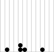
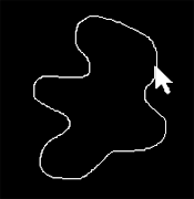
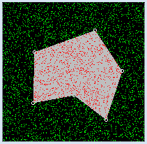
The Principality of Monaco is world famous for its casino in the Monte Carlo district. The casino has not only been an attraction for celebrities for the past 150 years, but also for mathematicians who try to analyze the games and develop winning strategies. The computer is much better for testing these strategies and is actually better than the real game, because you do not loose any money with computer experiments as you do in the real games. In the following "game", you throw points on a square area where there is a polygon. As an illustration, you can see the points as raindrops. As usual when it rains, there are always roughly about the same amount of drops in each unit area. So, the drops are uniformly distributed. You let a certain number of raindrops fall and then count how many of them fall onto the area of the polygon. It is obvious that the number will increase with an increasing surface area of the polygon, and that on average, it will be proportional to the surface area. For example, if you let drops fall onto a polygon with a surface area ¼ the size of the area of the surrounding square it will likely collect (on average) ¼ of all the raindrops. Once you have realized this, you can conversely find out the area by counting the number of the drops. Isn't this convenient?
from gpanel import * from random import random NB_DROPS = 10000 def onMousePressed(x, y): if isLeftMouseButton(): pt = [x, y] move(pt) circle(0.5) corners.append(pt) if isRightMouseButton(): wakeUp() def go(): global nbHit setColor("gray") fillPolygon(corners) setStatusText("Working. Please wait...") for i in range(NB_DROPS): pt = [100 * random(), 100 * random()] color = getPixelColorStr(pt) if color == "black": setColor("green") point(pt) if color == "gray" or color == "red": nbHit += 1 setColor("red") point(pt) setStatusText("All done. #hits: " + str(nbHit) + " of " + str(NB_DROPS)) makeGPanel(0, 100, 0, 100, mousePressed = onMousePressed) addStatusBar(30) setStatusText("Select corners with left button. Start dropping with right button") bgColor("black") setColor("white") corners = [] nbHit = 0 putSleep() go() |
MEMO |
When you click with the left mouse button you are saving the vertices of the polygon into a list corners and drawing small circles as marks. The actual rain simulation is performed in the function go(). It begins when you click the right mouse button and lasts for a certain amount of time. You make the falling raindrops visible with different colored points. If you directly call go() in the pressCallback(), as it might seem straightforward, you will see nothing until the simulation ends. The reason is that the system prevents refreshing the graphics in a mouse callback for system-intrinsic reasons. So if you want to visualize a longer-lasting action in a callback, it must happen in another part of the program. Often the main block of the program is used for this purpose. The execution is temporarily halted with putSleep(). The press event awakens the sleeping main program with wakeUp() and the simulation will be carried out with the call go(). Callbacks must always return quickly. Therefore, no long-lasting actions should be executed there. To find out if a raindrop has fallen onto the gray colored polygon area, use the following trick: You get the color of the point of impact with getPixelColorStr(). If it is the color gray (or red if another drop has already fallen there), you increase nbHit by 1 and color the point red. You can test the procedure by generating some simple polygons (e.g. rectangles, triangles) and then by measuring the screen with a ruler. You will then realize that you need a lot of raindrops in order to obtain a reasonably accurate result [more... For 1 decimal place better accuracy (factor of 10), you need 100 times more points]. |
CHAOS GAME |
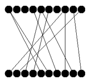
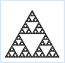
It might at first seem surprising that you can create regular patterns with random experiments. This has to do with the compensation of statistical fluctuations for large numbers. In 1988 Michael Barnsley invented the following algorithm based on Chaos theory, which builds on a random selection of the vertices of a triangle:
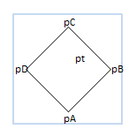
from gpanel import * from random import randint MAXITERATIONS = 100000 makeGPanel(0, 10, 0, 10) pA = [1, 1] pB = [9, 1] pC = [5, 8] triangle(pA, pB, pC) corners = [pA, pB, pC] pt = [2, 2] title("Working...") for iter in range(MAXITERATIONS): i = randint(0, 2) pRand = corners[i] pt = getDividingPoint(pRand, pt, 0.5) point(pt) title("Working...Done") |
MEMO |
If you need a random object, you can join all of the objects in a list and pick an object out of it at a random index. It is quite amazing that you can create a regular figure (called Sierpinski triangle) with randomly selected points. |
EXERCISES |
|