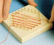
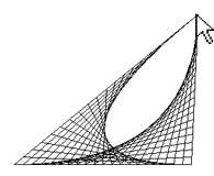
3.8 STRING ART
![]()
INTRODUCTION |
Instead of creating the thread graphic yourself, you can also instruct a machine to do it. This would require the machine to not only understand the instructions but then to also translate these instructions into an action, for example using a robot arm to pull the strings or record the strings on a screen. Such an instruction manual for a machine is also called an algorithm. You can first formulate the algorithm as a “craft” instruction understandable in colloquial language. Since it is desirable that the machine produces the exact same pattern on each pass, the algorithm must be formulated so precisely that the machine knows exactly what to do at every step. Programming languages were invented for this and that is why you learn to program, since in the natural languages there is no such unambiguity. |
POINTS AS LISTS |
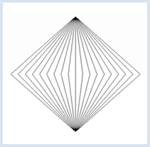
In geometry, you can write P(x, y) for a point, where x and y are the coordinates. In the program, we can pack the two numbers x and y into a data structure, called a list. We write p = [x, y]. The geometric point P(0, 8) is thus modeled by the list p = [0, 8] . You can access the individual components of a list with an index with a count starting at 0. You have to write the index in a set of square brackets, so p[0] for the x-coordinate, and p[1] for the y-coordinate. The nice thing is that all of the graphic functions of the GPanel are "list conscious" because they also work with point lists instead of x-y-coordinates. Your program models the pulling of threads from nail A around 19 nails at the coordinates on the x-axis to nail B, and back again. You can even incorporate a delay() which causes the stringing to take a longer time that is graspable by humans. from gpanel import * DELAY = 100 def step(x): p1 = [x, 0] draw(p1) delay(DELAY) draw(pB) delay(DELAY) p2 = [x + 1, 0] draw(p2) delay(DELAY) draw(pA) delay(DELAY) makeGPanel(-10, 10, -10, 10) pA = [0, 8] pB = [0, -8] move(pA) for x in range(-9, 9, 2): step(x) |
MEMO |
|
The data must also be structured conveniently in the implementation of an algorithm. Our geometric points are modeled as a list with two elements (x- and y-coordinates). The choice of the data structure significantly affects the program. Niklaus Wirth, a famous computer science professor at the ETH Zürich, aptly said: program = algorithm + data structure [Ref.] |
PROGRAMMING IS AN ART |
|
MEMO |
|
An algorithm can be implemented in various ways that differ in length of code and duration of the execution of the program. We also speak of more elegant and less elegant programs. Just remember that it is not enough for a program to produce a correct result, but it should also be written elegantly. Consider programming an art! |
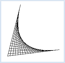
ELEGANT THREAD GRAPHIC ALGORITHMS |
from gpanel import * makeGPanel(0, 100, 0, 100) pA = [10, 10] pB = [90, 20] pC = [30, 90] line(pA, pB) line(pA, pC) r = 0 while r <= 1: pX1 = getDividingPoint(pA, pB, r) pX2 = getDividingPoint(pA, pC, 1 - r) line(pX1, pX2) r += 0.05 delay(300) |
MEMO |
|
Library functions such as getDividingPoint() can greatly simplify a program. For certain well-defined tasks, you should use existing library functions that you know from your programming experience here, taken from documentations, or from what you can find on the Web. Mathematically, the resulting curve is a quadratic Bézier curve. You can draw it with the function quadraticBezier(pB, pA, pC), where pB and pC are the endpoints, and pA is the control point of the curve. |
MOUSE CONTROLLED THREAD GRAPHICS |
In order to create the graphics, you use the function updateGraphics() which is called by the mouse callbacks. Every time you delete the entire graphics window and then recreate it with point A at the current location of the mouse cursor. from gpanel import * def updateGraphics(): clear() line(pA, pB) line(pA, pC) r = 0 while r <= 1: pX1 = getDividingPoint(pA, pB, r) pX2 = getDividingPoint(pA, pC, 1 - r) line(pX1, pX2) r += 0.05 def myCallback(x, y): pA[0] = x pA[1] = y updateGraphics() makeGPanel(0, 100, 0, 100, mousePressed = myCallback, mouseDragged = myCallback) pA = [10, 10] pB = [90, 20] pC = [30, 90] updateGraphics() |

MEMO |
|
You can also deal with two different events, here the press event and the drag event, using the same callback. |
EXERCISES |
|
EXTRA MATERIAL |
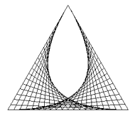
BÉZIER CURVES |
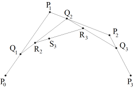
You can easily implement the algorithm into a program if you implement the points as lists and call the function getDividingPoint() several times. from gpanel import * makeGPanel(0, 100, 0, 100) pt1 = [10, 10] pc1 = [20, 90] pc2 = [70, 70] pt2 = [90, 20] setColor("green") line(pt1, pc1) line(pt2, pc2) line(pc1, pc2) r = 0 while r <= 1: q1 = getDividingPoint(pt1, pc1, r) q2 = getDividingPoint(pc1, pc2, r) q3 = getDividingPoint(pc2, pt2, r) line(q1, q2) line(q2, q3) r2 = getDividingPoint(q1, q2, r) r3 = getDividingPoint(q2, q3, r) line(r2, r3) r += 0.05 setColor("black") #cubicBezier(pt1, pc1, pc2, pt2) |
MEMO |
|
A cubic Bézier curve is defined by 4 points. You can draw one in GPanel with the function cubicBezier(). The current drawing color and line thickness will be used. |
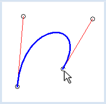
INTERACTIVE CURVE DESIGN |
It is also important that you know which of the points you have just grabbed. You store this information in the variable active: if none of the points are grabbed it has the value -1, otherwise its value corresponds to the index of the corresponding point. from gpanel import * def updateGraphics(): # erase all clear() # draw points lineWidth(1) for i in range(4): move(points[i]) if active == i: setColor("green") fillCircle(2) setColor("black") circle(2) # draw tangents setColor("red") line(points[0], points[1]) line(points[3], points[2]) # draw Bezier curve setColor("blue") lineWidth(3) cubicBezier(points[0], points[1], points[2], points[3]) def onMouseDragged(x, y): if active == -1: return points[active][0] = x points[active][1] = y updateGraphics() def onMouseReleased(x, y): active = -1 updateGraphics() def onMouseMoved(x, y): global active active = near(x, y) updateGraphics() def near(x, y): for i in range(4): rsquare = (x - points[i][0]) * (x - points[i][0]) + (y - points[i][1]) * (y - points[i][1]) if rsquare < 4: return i return -1 pt1 = [20, 20] pc1 = [10, 80] pc2 = [90, 80] pt2 = [80, 20] points = [pt1, pc1, pc2, pt2] active = -1 makeGPanel(0, 100, 0, 100, mouseDragged = onMouseDragged, mouseReleased = onMouseReleased, mouseMoved = onMouseMoved) updateGraphics() |
MEMO |
|
There are also complicated data structures such as lists whose elements are again lists. For example, you can address the x-coordinate of P1 using the points[1][0], thus with double brackets. Today, Bézier curves are important design tools in the CAD domain [Ref.] |
EXERCISES |
|