10.7 INFORMATION & ORDER
![]()
INTRODUCTION |
Even though the word information is used often, it is not that easy to grasp the concept precisely and to make it measurable. In daily life, more information is associated with more knowledge and it is said that a person A informed in a certain thing knows more than an uninformed person B. In order to measure how much more information A has than B (or team B), or the lack of information of B with respect to A, you best imagine a TV quiz show. Person or team B has to find something out that only person A knows, for example their profession. Thereby B asks questions that A has to answer with a Yes or a No. The rules are as follows: The lack of information I of B in relation to A (in bits) is the number of questions with Yes/No answers that B (on average and at an optimal asking strategy) has to ask in order to have the same knowledge about a certain thing as A has. |
NUMBER GUESSING GAME |
You can enact such a guessing game in your classroom (or just in your head) as follows: Your classmate Judith is sent out of the room. One of the remaining W = 16 classmates receives a "desired" object, such as a bar of chocolate. After Judith is called back into the classroom, you and your classmates know who has the chocolate, but Judith does not. How big is her lack of information? For the sake of simplicity, the classmates are numbered from 0 to 15 and Judith can now ask everyone questions in order to find out the secret number of the classmate with the chocolate. The less questions she asks, the better. One possibility would be for her to ask any random number: "Is it 13?". If the answer is No, she asks a different number.
If the secret number is 0, then 1 question is needed to find the answer; if the secret number is 1, 2 questions are needed, etc. If the secret number is 14, then 15 questions are needed, but when the secret number is 15, again only 15 questions are needed since it is the last possible option. The program plays the game 100,000 times and counts the number of questions it takes in each case until the secret number is determined. Those numbers are added up to finally determine the average. from random import randint sum = 0 z = 100000 repeat z: n = randint(0, 15) if n != 15: q = n + 1 # number of questions else: q = 15 sum += q print("Mean:", sum / z) With this strategy, Judith would need to ask an average of 8.43 questions. That is quite a lot. But since Judith is clever, she decides to use a much better strategy. She asks them: "Is it a number between 0 and 7?" (limits included). If the answer is Yes, she divides the area into two equal parts again and asks: "Is the number between 0 and 3?". If the answer is again Yes, she asks "Is it 0 or 1?" and if the answer is Yes she asks: "Is it 0?". No matter what the response, she now knows the number. With this "binary" (questioning) strategy and when W = 16, Judith always has to ask exactly 4 questions and therefore 4 is the average number of questions asked. This shows us that the binary (questioning) strategy is optimal and the information about the owner of the chocolate bar has thus the value I = 4 bit.
|

MEMO |
|
As you can easily find out, with W = 32 numbers the information amounts to I = 5 bit, and with W = 64 numbers I = 6 bit. So apparently we get 2I = W or I = ld(W). It also does not need to be a number that one is searching for, but rather it can consist of any one state that has to be found out from W (equally probable) number of states. So the information at the knowledge of a state from W equally probable states is |
INFORMATION CONTENT OF A WORD |
Since the W states are equally likely, the probability of the states is p = 1/W. You can also write the information as follows: I = ld(1/p) = -ld(p) You certainly know that the probabilities of certain letters in a spoken language differ greatly. The following table shows the probabilities for the English language [more... The values depend on the type of text. The numbers correspond to a literary text].
It is certainly not the case that the probability of a letter in a word is independent of the letters of the words you already know and the context in which the word appears. However, if we make this simple assumption, then the probability p of a 2-letter combination with the individual probabilities p1 and p2 is, according to the product rule, p = p1 * p2 and for the information:
or for arbitrarily many letters:
In your program, you can enter a word and you will get the information content of the word as an output. For this you should download the files with the letter frequencies in German, English, and French from here and copy them to the directory where your Python program is. from math import log f = open("letterfreq_de.txt") s = "{" for line in f: line = line[:-1] # remove trailing \n s += line + ", " f.close() s = s[:-2] # remove trailing , s += "}" occurance = eval(s) while True: word = inputString("Enter a word") I = 0 for letter in word.upper(): p = occurance[letter] / 100 I -= log(p, 2) print(word, "-> I =", round(I, 2), "bit")
|
MEMO |
|
The data are saved in the text file line by line in the format 'letter' : percentage. In Python, a dictionary is well suited as a data structure for this. In order to convert the data information to a dictionary, the lines are read and packed into a string in standard dictionary format {key : value, key : value,...}. This string is interpreted as a line of code with eval() and a dictionary is created. As you can find out with your program, the information content of words with rare letters is greater. However, the information content determined this way has nothing to do with the importance or personal relevance of a certain word in a certain context, or in other words whether the information connected to the word is trivial for you or of crucial importance. It is far beyond the capabilities of today's information systems to determine a measure for this. |
EXERCISES |
|
ADDITIONAL MATERIAL |
THE RELATIONSHIP BETWEEN DISORDER AND ENTROPY |
There is an extremely interesting relationship between the information that we have about a system and the order of the system. For example, the order is certainly much greater when all students in a classroom are sitting at their desks, than when they are all moving around randomly in the room. In the disordered state, our lack of information of where each individual person is located is very high, thus we can use this lack of information as a measure of disorder. For this, one defines the concept of entropy:
As you can determine, systems left to their own resources have the tendency to move from an ordered to a disordered state. For example:
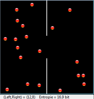
The module gamegrid is used for the animation. The particles are modeled in the class Particle that is derived from the class Actor. You can move the particles using the method act(), which is automatically called in each simulation cycle. The collisions are handled with collision events. For this, derive the class CollisionListener from GGActorCollisionListener and override the method collide(). This procedure is the same as what you saw in chapter 8.10 on Brownian Movement. The 20 particles are then divided into 4 different velocity groups. Since the velocities are switched between particles that collide, the total energy of the system remains constant, i.e. the system is closed. from gamegrid import * from gpanel import * from math import log # =================== class Particle ==================== class Particle(Actor): def __init__(self): Actor.__init__(self, "sprites/ball_0.gif") # Called when actor is added to gamegrid def reset(self): self.isLeft = True def advance(self, distance): pt = self.gameGrid.toPoint(self.getNextMoveLocation()) dir = self.getDirection() # Left/right wall if pt.x < 0 or pt.x > w: self.setDirection(180 - dir) # Top/bottom wall if pt.y < 0 or pt.y > h: self.setDirection(360 - dir) # Separation if (pt.y < h // 2 - r or pt.y > h // 2 + r) and \ pt.x > self.gameGrid.getPgWidth() // 2 - 2 and \ pt.x < self.gameGrid.getPgWidth() // 2 + 2: self.setDirection(180 - dir) self.move(distance) if self.getX() < w // 2: self.isLeft = True else: self.isLeft = False def act(self): self.advance(3) def atLeft(self): return self.isLeft # =================== class CollisionListener ========= class CollisionListener(GGActorCollisionListener): # Collision callback: just exchange direction and speed def collide(self, a, b): dir1 = a.getDirection() dir2 = b.getDirection() sd1 = a.getSlowDown() sd2 = b.getSlowDown() a.setDirection(dir2) a.setSlowDown(sd2) b.setDirection(dir1) b.setSlowDown(sd1) return 5 # Wait a moment until collision is rearmed # =================== Global sections ================= def drawSeparation(): getBg().setLineWidth(3) getBg().drawLine(w // 2, 0, w // 2, h // 2 - r) getBg().drawLine(w // 2, h, w // 2, h // 2 + r) def init(): collisionListener = CollisionListener() for i in range(nbParticles): particles[i] = Particle() # Put them at random locations, but apart of each other ok = False while not ok: ok = True loc = getRandomLocation() if loc.x > w / 2 - 20: ok = False continue for k in range(i): dx = particles[k].getLocation().x - loc.x dy = particles[k].getLocation().y - loc.y if dx * dx + dy * dy < 300: ok = False addActor(particles[i], loc, getRandomDirection()) delay(100) # Select collision area particles[i].setCollisionCircle(Point(0, 0), 8) # Select collision listener particles[i].addActorCollisionListener(collisionListener) # Set speed in groups of 5 if i < 5: particles[i].setSlowDown(2) elif i < 10: particles[i].setSlowDown(3) elif i < 15: particles[i].setSlowDown(4) # Define collision partners for i in range(nbParticles): for k in range(i + 1, nbParticles): particles[i].addCollisionActor(particles[k]) def binomial(n, k): if k < 0 or k > n: return 0 if k == 0 or k == n: return 1 k = min(k, n - k) # take advantage of symmetry c = 1 for i in range(k): c = c * (n - i) / (i + 1) return c r = 50 # Radius of hole w = 400 h = 400 nbParticles = 20 particles = [0] * nbParticles makeGPanel(Size(600, 300)) window(-6, 66, -2, 22) title("Entropy") windowPosition(600, 20) drawGrid(0, 60, 0, 20) makeGameGrid(w, h, 1, False) setSimulationPeriod(10) addStatusBar(20) drawSeparation() setTitle("Entropy") show() init() doRun() t = 0 while not isDisposed(): nbLeft = 0 for particle in particles: if particle.atLeft(): nbLeft += 1 entropy = round(log(binomial(nbParticles, nbLeft), 2), 1) setStatusText("(Left,Right) = (" + str(nbLeft) + "," + str(nbParticles-nbLeft)+ ")"+" Entropie = "+str(entropy)+" bit") if t % 60 == 0: clear() lineWidth(1) drawGrid(0, 60, 0, 20) lineWidth(3) move(0, entropy) else: draw(t % 60, entropy) t += 1 delay(1000) dispose() # GPanel
|
MEMO |
|
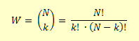
When seen from the outside (macroscopically), a state is determined by the number k of particles in the right part, and thus N - k in the left part. A macroscopic observation lacks the precise knowledge, which k of the N numbered particles are on the right. According to combinatorics there are such possibilities. The lack of information is therefore
The temporal process is plotted in a GPanel graphic. You can clearly see that the particles distribute themselves throughout the entire container over time, but there is also a chance that all particles end up again in the left half. The probability of this decreases rapidly with an increasing number of particles. The 2nd law thus relies on a statistical property of multiple-particle systems. Since the reverse process is not observed, these processes are called irreversible. However, there are indeed processes that passed from disorder to order. For this, they need an "ordering constraint" [more... This is known as a "enslavement"].Some examples are:
These processes decrease the disorder, and therefore the entropy, so that structures gradually become visible from chaos. |
EXERCISES |
|