![]()
INTRODUCTION |
Sequences of numbers have fascinated people for a long time. Already in ancient times around 200 B.C. Archimedes had approximated the number of Pi through a sequence of numbers that he found by calculating the perimeters of regular polygons with increasingly many vertices that fit into a circle. It was already clear to him then that the circle could be regarded as a border-line case of a regular polygon with infinitely many vertices. Therefore, he found that the perimeters of the polygons had to strive towards the circumference of the circle. A sequence of numbers consists of the numbers a0, a1, a2, etc., thus of the terms an with index n = 0, 1, 2, etc. (sometimes it begins with n = 1). A formation rule clearly determines how big each number is. If ak is defined for any natural number, however large it may be, we speak of an infinite sequence of numbers. The principle can be specified as an explicit expression of n. However, a term may also be calculated from previous terms of the series (recursive rule). In this case, the start values must also be known. A convergent sequence has a very descriptive property: there is a unique number g called a limit that the terms gradually approach, which means that you can choose any arbitrarily small neighborhood interval of g so that none of the following terms fall outside of the chosen interval starting at a definite n. You can imagine the neighborhood as a house around the limit: before that, the sequence may leap around wildly, however after a certain n all terms of the sequence end up in the house no matter how small it may be. 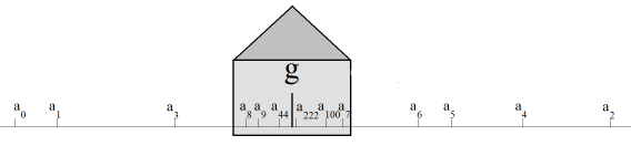 Number sequences can be studied experimentally using the computer. In order to illustrate them, you use various graphical representations: You can, for instance, similar to the above illustration, draw all terms as points or lines and analyze whether there is a limit point. However, you can also investigate how the sequence behaves for large values of n by representing it as a two dimensional graph where the n are on the x-axis and the an on the y-axis. |
THE HUNTER AND HIS DOG |
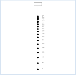
A hunter walks with his dog with the velocity u = 1 m/s to their hunting lodge d = 1000 m away. However, since the hunter walks too slowly for the dog, the dog proceeds as follows: It runs alone at its own velocity u = 20 m/s to the hunting lodge, turns around, and then runs back to its owner. As soon as it reaches its owner, it turns around again and runs back to the hunting lodge, and then continues this behavior.
From this, you can deduce the following relationship with little knowledge of Algebra:
As you might have expected, the numbers an pile up against the limit number 1000. from gpanel import * u = 1 # m/s v = 20 # m/s d = 1000 # m a = 0 # hunter h = 0 # dog c = 2 * u / (u + v) it = 0 makeGPanel(-50, 50, -100, 1100) title("Hunter-Dog problem") line(0, 0, 0, 1000) line(-5, 1000, 5, 1000) line(-5, 1050, 5, 1050) line(-5, 1000, -5, 1050) line(5, 1000, 5, 1050) while not isDisposed(): move(0, a) fillCircle(1) text(5, a, str(int(a))) getKeyWait() da = c * (d - a) dh = 2 * (d - a) - da h += dh a += da it += 1 title("it = " + str(it) + "; hunter = " + str(a) + " m; dog = " + str(h) + " m")
|
MEMO |
|
One says that the number sequence an converges and that its limit value is 1000. Think about why this problem is of a theoretical nature. It corresponds to the ancient anecdote where Achilles was invited to race with a turtle. Since he was ten times faster than the turtle, the turtle would have gotten a head start of 10 meters. Achilles refused to compete because in his opinion, he had no chance to catch up with the turtle. So, he argued: In the time that he needed for the first 10 meters, the turtle would have already advanced 1 meter. In the time that he needed for this one meter, the turtle would already be 10 cm further. In the time that he then needed for these 10 cm, the turtle would already be another 1 cm further, and so forth. What do you think about this? |
BIFURCATION DIAGRAM (FEIGENBAUM BIFURCATION) |
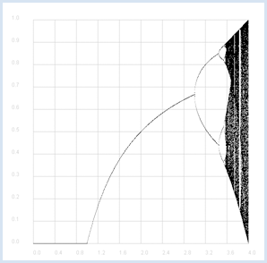
You got to know the logistic growth in the context of population dynamics. The population size xnew in the next generation is calculated from its current size x from a quadratic relationship. The relationship is simplified in the following (parameter r can be arbitrarily chosen) :
from gpanel import *

def f(x, r):
     return r * x * (1 - x)

makeGPanel(-0.6, 4.4, -0.1, 1.1)
title("Tree Diagram")
drawGrid(0, 4.0, 0, 1.0, "gray")
for z in range(1001):
    r = 4 * z / 1000
    a = 0.5
    for i in range(1001):
        a = f(a, r)
        if i > 500:
            point(r, a)
|
MEMO |
|
In the experiment, you detect the limit points of the sequence for a certain r. Based on a computer simulation, you can establish the following assumptions: For r < 1 there is a limit point at 0 and so the sequence converges to 0. The sequence likewise converges in the area between 1 and 3. There are initially two and later more limit points for an even larger r, but the sequence no longer converges. For even larger values of r the sequence chaotically jumps back and forth. |
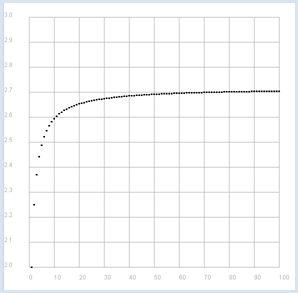
THE EULER NUMBER |
from gpanel import *

def a(n):
     return (1 + 1/n)**n

makeGPanel(-10, 110, 1.9, 3.1)
title("Euler Number")
drawGrid(0, 100, 2.0, 3.0, "gray")
for n in range(1, 101):
    move(n, a(n))
    fillCircle(0.5)
|
MEMO |
This is a case of the Euler number e, arguably one of the most famous numbers ever. |
QUICK CONVERGING SEQUENCES FOR THE CALCULATION OF PI |
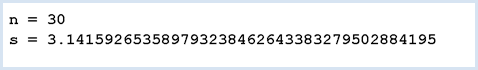
The calculation of πfor as many digits as possible poses a challenge since ancient times. A sum formula was discovered only in 1995 by the mathematicians Bailey, Borwein and Plouffe called the BBP formula. They proved that you can get exactly π as the limit value of a sequence whose n-th term is the sum from k = 0 to k = n of:
Your program uses the Python modulle decimal which provides the decimal numbers with a high level of accuracy. The constructor creates such a number from an integer or a float where common mathematical operation signs can be used directly. You can set the accuray with getcontext().prec. This roughly corresponds to the number of decimal places used. Each time a button is pressed, your program calculates the next term of the sequence and represents the value in a EntryDialog.
from entrydialog import *
from decimal import *
getcontext().prec = 50

def a(k):
    return 1/16**Decimal(k) * (4 / (8 * Decimal(k) + 1) - 2
    / (8 * Decimal(k) + 4) - 1
    / (8 * Decimal(k) + 5) - 1 / (8 * Decimal(k) + 6))

inp = IntEntry("n", 0)
out = StringEntry("Pi")
pane0 = EntryPane(inp, out)
btn = ButtonEntry("Next")
pane1 = EntryPane(btn)
dlg = EntryDialog(pane0, pane1)
dlg.setTitle("BBP Series - Click Next")
n = 0
s = a(0)
out.setValue(str(s))
while not dlg.isDisposed():
    if btn.isTouched():
       n = inp.getValue()
       if n == None:
           out.setValue("Illegal entry")
       else:
           n += 1
           s += a(n)
           inp.setValue(n)
           out.setValue(str(s))
|
MEMO |
|
At just 40 iterations the displayed number for π no longer changes. The program ends when you close the display window, since isDisposed() is True. |
EXERCISES |
|
ADDITIONAL MATERIAL |
ITERATIVE SOLUTION OF AN EQUATION |
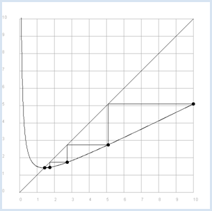
from gpanel import *

def f(x):
    return 1 / 2 * (x + 2 / x)

makeGPanel(-1, 11, -1, 11)
title("Iterative square root begins at x = 10. Press a  key...")
drawGrid(0, 10, 0, 10, "gray")

for i in range(10, 1001):
    x = 10 / 1000 * i
    if i == 10:
        move(x, f(x))
    else:
        draw(x, f(x))

line(0, 0, 10, 10)

x = 10
move(x, f(x))
fillCircle(0.1)
it = 0
while not isDisposed():
    getKeyWait()
    it += 1
    xnew = f(x)
    line(x, f(x), xnew, f(x))
    line(xnew, f(x), xnew, f(xnew))
    x = xnew
    move(x, f(x))
    fillCircle(0.1)
    title("Iteration " + str(it) + ": x = " + str(x))
|
MEMO |
You can clearly see that with each press of the key the points move quickly towards the point of intersection. Just a few iterations results in a solution with 10 digits of accuracy. |